3D Analysis: Modifiers

Modifiers are special functions to improve or optimize your scan images based on its recorded measuring values. Figure 1 shows the Modifiers Panel that is located in the Right Sidebar of the Visualizer 3D Studio software.

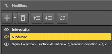
**Figure 1:** Modifiers Panel of the Right Sidebar

On top of the panel is a toolbar and right beneath the list of added modifiers. This list contains all created modifiers, even if they are not active (which is indicated by the strikethrough eye symbol).

The toolbar contains following buttons:

	Add Modifier Push this button to add a new modifier that should be applied to your current scan image. The popup menu that appears provides all modifiers that are explained in the subsequent subsection.
	Delete Modifier Push this button to delete the selected modifier from the list of all added modifiers.
	Move Modifier Upwards Push this button to move the selected modifier one level up. This will change the order of the modifiers and will also change the outcome when the modifiers are applied to the current scan image.
	Move Modifier Downwards Push this button to move the selected modifier one level down. This will change the order of the modifiers and will also change the outcome when the modifiers are applied to the current scan image.
	Refresh List Push this button to re-apply all modifiers to the raw data of the scan image. This might be necessary if you changed the status of a modifier from active to inactive or vice versa.

Modifiers

You can apply as much modifiers as needed. The order of the modifiers is always from top to bottom, so the first modifier is applied first and then all the other modifiers in the list are applied to the scan image. Please keep in mind that a different order leads to different results.

You can also toggle the status of each modifier by clicking the eye icon. Only active or enabled modifiers are applied to the scan image to change its corresponding data. All inactive or disabled modifieres are skipped.

There are four modifiers in total, that can be used to be applied to your scan images:

Interpolation
The Interpolation modifier recalculates all scan values to smooth out any spikes that may occur while measuring an area.
Subdivision
The Subdivision modifier adds additional scan values (calculated by specific algorithms) into the data grid. This gives a much higher resolution of the scan image.
Signal Correction
The Signal Correction modifier is used to remove error signals or erroneous scan values that might result from wireless interferences or wrong handling of the metal detector like changing the height of the probe while scanning.
Rotational Correction
The Rotational Correction modifier has been made to correct errors based on the scan mode (Zig-Zag or Parallel) of a conducted measurement and its following data transfer.

All of the modifiers are explained in more detail in the following subsections.

Interpolation

With the Interpolation modifier you can improve the representation of the scan image and eliminate certain irregularities in the measurement data. It is also possible to check potential objects regarding mineralization.

Figure 2 shows the scan image before Interpolation and figure 3 shows the same scan image after applying the Interpolation modifier.

The Interpolation modifier is a suitable tool to distinguish real objects from mineralization. When there is a signature of a real metallic object inside the scan image, it will also be visible after using the Interpolation modifier several times. It will also keep the same position, size and shape. If the anomaly disappears or got split into more parts or change its position radically, than it is probably a natural mineralization of the ground.

If you repeat the interpolation process too often, also real objects will disappear from the scan image.

Subdivision

The Subdivision modifier can also be used to smoothen out the spiky signals but furthermore it generates additional scan values to increase the resolution of the scan image.

Figure 4 shows a scan image without any modifier applied, whereas figure 5 shows the same scan image with applied Subdivision modifier.

The chosen wireframe representation of the scan image clearly shows that the number of measured values has been increased by applying the Subdivision modifier.

Please keep in mind that this modifier adds additional data that has not been measured in the field. It is always recommended to record as much real world data as possible. Applying this modifier too often might also slow down your computer, because it has to process more scan values.

Signal Correction

There are very different environmental influences, that can affect the graphical representation of the measurement in a negative way. The Signal Correction modifier is used to eliminate error signals from the graphical representation. Such error signals can occur by wrong handling of the detector or by small but highly responsive metal targets close to the ground surface.

When selecting the Signal Correction modifier the configuration dialog from figure 6 appears on the screen.

In the dialog there are two main options available:

Correct the signal under the crosshairs
With this option checked, only the scan value at the crosshairs (3D cursor) will be processed and corrected.
Correct all signals (Automatic Mode)
Check this option to correct all signals of the scan image that match the following subsettings:
- Average Deviation from Normal Surface Value
  This value specifies the minimum deviation of a scan value to the Normal Surface Value (Ground Value). The value "0" means no deviation at all.
- Average Deviation from Surrounding Values
  This value specifies the minimum deviation of a scan value to its adjoining scan values. The value of "0" means no deviation at all.

Figure 7 shows a scan image including two error signals. Often the whole scan image will be colored red or blue completely but the error signals. Another very typical characteristic of an error signal is that it consists of mostly one scan value with an extreme deviation from the surrounding values.

Figure 8 shows the same scan image as figure 7, but after applying the Signal Correction modifier. Now the real anomalies become visible, that were hidden before.

Strong signals (e.g. high responsive metals close to the surface) hide weaker signal (e.g. deeper metal objects or cavities).

Rotational Correction

The last modifier that needs to be described is the Rotational Correction modifier, that can be used if the scan mode (Parallel or Zig-Zag) of the actual measurement and the data transfer has been mismatched.

Example: You conducted a measurement in Parallel scan mode but you transferred the scan data by selecting the scan mode Zig-Zag.

In that kind of situation you can use the Rotational Correction modifier to fix the mismatch afterwards.

Figure 9 shows a scan image that was recorded in Parallel scan mode but conducted in Zag-Zag. The typical indications are the red/blue stripes. The scan shows no anomaly that indicates any kind of hidden object.

Figure 10 shows the same scan image after applying the Rotational Correction modifier. Now there is some kind of object anomaly visible.

At this point it is recommended to repeat the measurement to get high quality real world data of the scan area.

Tags: Interpolation Modifiers Rotational Correction Signal Correction Subdivision